Cirrhosis Survival Analysis

A clinical research group had follow-up data on patients with cirrhosis and a question that looks simpler than it is: which patient characteristics are associated with shorter survival? The tempting shortcut — comparing average follow-up time, or treating death as a yes/no flag — throws away the most important information in the cohort: when events happened, and which patients were still event-free when observation ended.

The question behind the data

The group wanted to describe survival in the cohort, identify candidate prognostic markers for further study, and compare an active treatment with a control group. Each of those is a different question. The third one mattered most to get right, because treatment was not randomly assigned and the data could not support a causal claim — however convenient that claim would have been.

What the cohort contained

A few hundred patients, twenty variables:

• Follow-up: days from registration to event or censoring, and a status variable distinguishing censored, death and transplant.
• Treatment: the assigned drug group.
• Demographics and clinical signs: age, sex, ascites, hepatomegaly, spider angiomata and edema.
• Laboratory markers: bilirubin, cholesterol, albumin, copper, alkaline phosphatase, SGOT, triglycerides, platelets and prothrombin time.
• Disease stage: histological stage.

With a sample this small, every parameter costs evidence. Flexible models with many terms would fit the noise and leave the group with conclusions that would not replicate.

The traps we designed around

• Censoring. Patients still alive at the end of follow-up are not "survivors" in the same sense as patients who completed the study. Dropping them biases survival upward; treating them as events biases it downward. Time-to-event methods use the partial information they contain.
• Competing events. A transplant removes the patient from the risk of death from cirrhosis, but it is not a death. We tested how sensitive the conclusions were to that choice instead of assuming the question away.
• Correlated markers. Bilirubin, albumin, prothrombin time and stage all move together. Putting them all into one model produces unstable coefficients that look precise and are not.
• Observational treatment. The drug group differed from the control group before treatment started. Any difference in survival is an association, and the analysis had to say so in the same font size as the rest of the findings.

How the analysis was built

1. Describe the censoring first. We started with how many patients had an event, how many were censored, and how much follow-up each group actually had. Survival analysis is only interpretable when this is on the table.
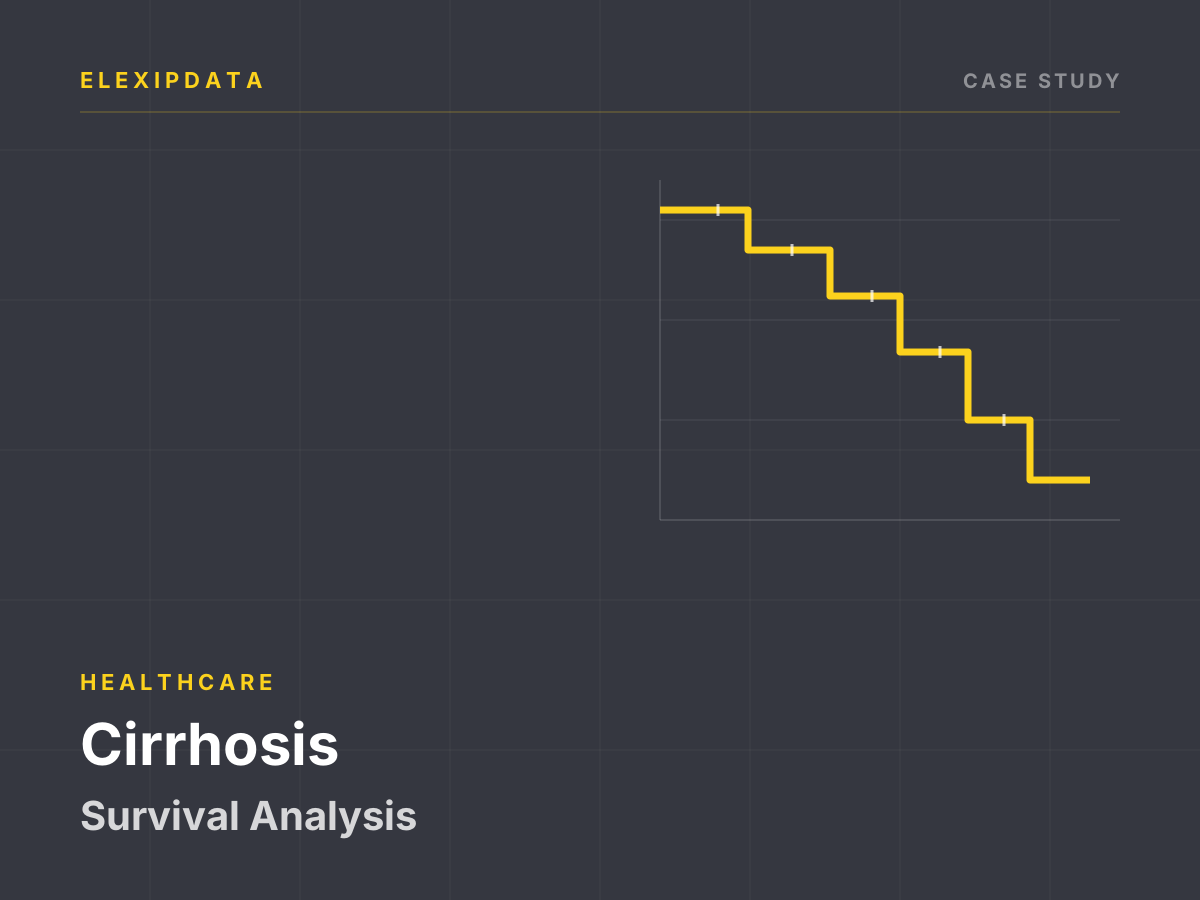
2. Plot before modelling. Kaplan-Meier curves by stage, edema and treatment group, with risk tables and log-rank tests, gave the group a picture of the data before any multivariable model.
3. Fit a Cox model with restraint. The multivariable model was restricted to clinically plausible, non-redundant markers. Proportional hazards were checked; where the assumption failed, we said so rather than reporting a coefficient that no longer meant what it appeared to mean.
4. Test the competing-risk sensitivity. The same questions were asked under a competing-risk framing. Where the conclusions held, confidence increased; where they did not, the limitation was reported.
5. Separate discrimination from calibration. Concordance was reported alongside calibration at clinically meaningful horizons. A model can rank patients correctly and still give misleading absolute risks.
6. Write the limitations as findings. The limitations section was treated as part of the result: what the cohort can support, what it cannot, and which questions need a larger or randomised study.

What the analysis changed

• The group gained a defensible survival description. Stage and key laboratory markers showed associations that held under sensitivity checks; weaker markers were reported as unresolved rather than promoted.
• The treatment comparison was correctly downgraded. It became hypothesis-generating evidence, not a reason to change practice — which protected the group from an overclaim in publication and peer review.
• The next study was easier to design. The analysis identified which markers were worth measuring in a larger cohort and how much follow-up would be needed to answer the treatment question properly.

What we delivered

• Kaplan-Meier curves with risk tables for stage, edema and treatment group.
• A Cox model summary with assumption checks and a plain-language interpretation of each retained marker.
• A sensitivity analysis for competing risks.
• A limitations section written for a clinical audience and a publication-ready methods description.

Where this applies

This method fits registries, hospital cohorts, clinical trials and any dataset where the outcome is an event with a date. The minimum inputs are a patient identifier, a start date, an event date or censoring date, an event-type indicator and the covariates of interest. The first deliverable is usually the censoring and competing-risk review — the step that decides whether the rest of the analysis can be trusted.

This is an illustrative case study using anonymized data with no patient-level information; it does not report results from a specific client engagement. It reflects our standard method for time-to-event analysis in clinical research.